1 + 1 + 5[1] 7This chapter introduces you to Stata, how to install it and the different ways to use it for statistical analysis. Stata is a powerful tool, but it remains a tool. The statistical concepts you learn are more important, and you will likely have to change the tools you use throughout your career. As a Brown University affiliate, you can download and install the software following instructions on this page. There are many versions of Stata, and you should install the latest version available. The code included in this book will work for version 17 and those more recent. Stata / IC should be sufficient for most of the
1.2 Stata syntax and Naming conventions
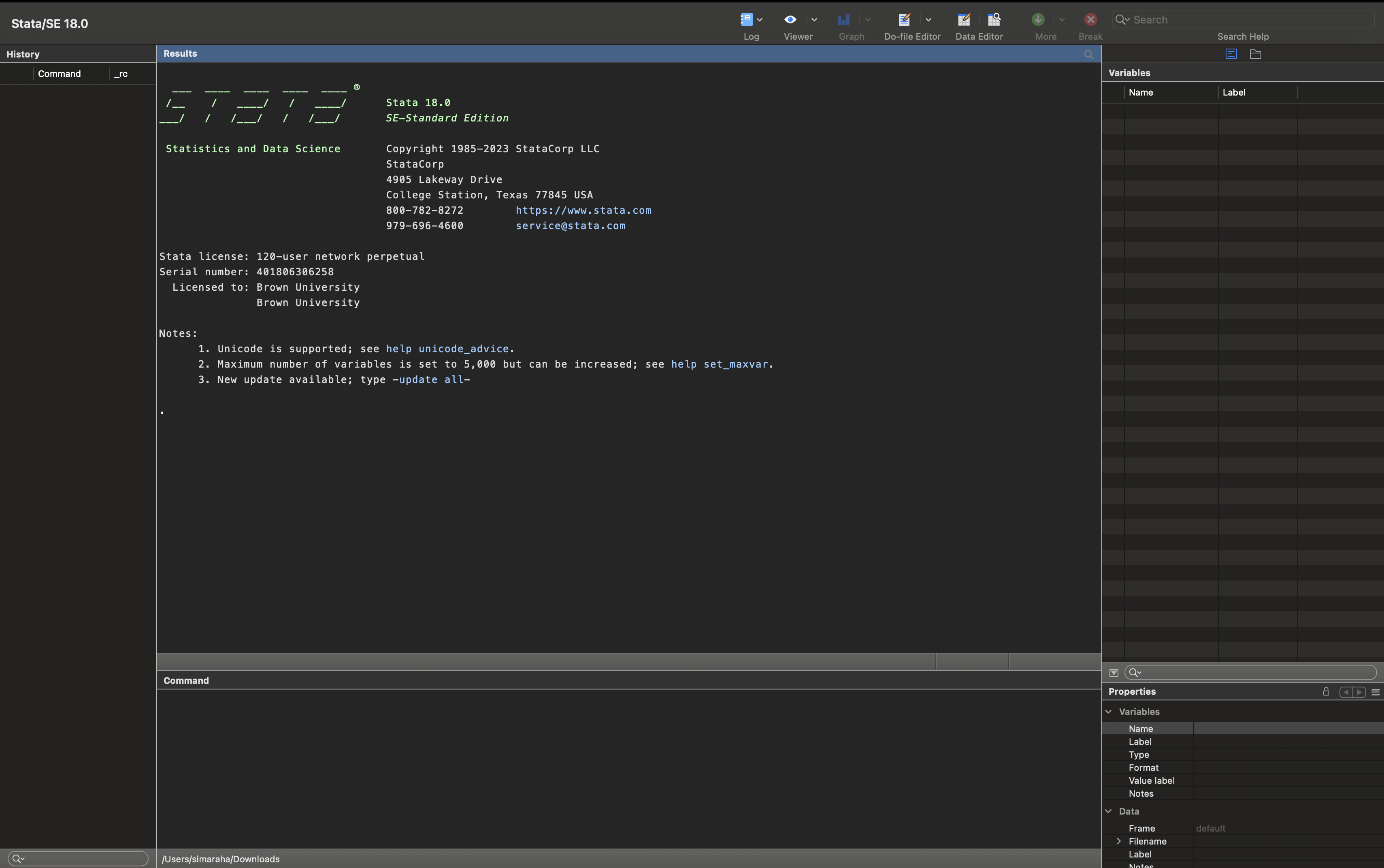
1.3 Using the command prompt
* ---------------------------------------------------------
* CLASS EXERCISE – UNIT 1
* Dataset: mcas_final_updated.dta
* Main task: practice basic Stata commands, descriptive
* statistics, and graphing distributions.
* ---------------------------------------------------------

* Load the dataset (adjust folder path if needed)
use "mcas_final_updated.dta", clear

* ---------------------------------------------------------
* 1. BASIC COMMANDS FOR VARIABLE: mathscore
* ---------------------------------------------------------

* Browse dataset (opens Data Browser)
browse

* Summary statistics: mean, sd, min, max
summarize mathscore

* Detailed summary: percentiles, variance, skewness, kurtosis, etc.
summarize mathscore, detail

* Stem-and-leaf plot
stem mathscore

* Boxplot
graph box mathscore, name(mathscorebox, replace)

* Histogram with frequencies
histogram mathscore, frequency name(mathscore, replace)

* ---------------------------------------------------------
* Saving graphs
* ---------------------------------------------------------

* Save graph in Stata's .gph format
graph save mathscore "dotmathscore.gph", replace

* Export histogram as .png
graph export "mathscore_hist.png", as(tif) width(2000) replace


* End of Part 1
* ---------------------------------------------------------

/* 2) Use the output from these commands to describe the distribution of mathscore in more detail.
How could you summarize what you see? Below, practice summarizing the univariate descriptive
statistics in no more than three sentences. (Remember to describe the following: unit of analysis,
central tendency, spread of the distribution, scale, skewness/symmetry, and atypical data points-
e.g., outliers).*/

/* 3) Now adapt this code for the ppe variable to produce univariate descriptive statistics and a
histogram. Below, practice summarizing the univariate descriptive statistics in no more than three
sentences.*/

* UNIVARIATE DESCRIPTIVE STATISTICS FOR PPE
* ---------------------------------------------------------

summarize ppe
summarize ppe, detail
stem ppe
graph box ppe, name(ppebox, replace)
histogram ppe, frequency name(ppehist, replace)

* Save graphs
graph save ppebox "doppebox.gph", replace
graph export "ppe_hist.png", as(tif) width(2000) replace
1.3.1 Make students use it as a calculator
1.4 Loading data
Download the dataset
You can download the dataset used in this chapter here:
```stata
use "mcas_final_updated.dta", clear
describe
```
1.4.1 Introduce an educational dataset – maybe OECD, NCES, open dataset Working Directory
1.4.2 Stata code count, describe, labels, etc.
1.5 Installing Packages
1.5.1 Give some examples to do
1.6 Tips and resources
1.6.1 Give some links to pages
1 + 1 + 5[1] 7